1. Introduction
Our society is moving increasingly towards algorithmic reliance for a range of decision problems. These decisions directly affect not only individuals but also society as a whole when they are adopted by organizations, some of which are fundamental, such as financial and educational institutions. This raises significant requirements on the trustworthiness and explainability of machine learning models. Among approaches, post-hoc explanations balance between transparency and safeguarding exploitative gaming behaviors. Post-hoc explanations aim to demonstrate why unfavorable decisions are made and how different the input should be so one can obtain a favorable outcome. Thus, these explanations can also be offered as recourses to benefit users, rather than being sole explanations for the system.
A recourse recommends the actions that an individual should take in order to receive an alternate algorithmic outcome. For example, consider an applicant who is rejected for a particular job, a recourse for a future success application may come in the form of personalized recommendations:
- Complete a 6-month full-stack engineer internship
- Score 60 more points in an ability test
However, decision systems could be updated frequently in practice due to data distribution shifts, rendering recommended recourses useless.
Following this line, our work focus on robust recourses, e.g., recourses that are effective at reversing the algorithmic outcome even under model shifts.
2. Bayesian Recourse
We consider a generic covariate space  and a binary predicted label
  , where class 0 denotes an unfavorable outcome while class 1 denotes a favorable one. Consider the joint random vector of covariate-label
  , then the class posterior probability of any input
  can be represented by the conditional random variable
  .
.
Bayesian Recourse
Given an input  , let
, let  be a neighborhood around . A Bayesian recourse
  is an alternative that minimizes the Bayesian posterior odds ratio
![\[x_{Bayes} \triangleq \underset{x \in \mathbb{X}}{\arg \min}~ \displaystyle \frac{\mathbb{P}( \hat{Y} = 0 | X = x)}{ \mathbb{P}( \hat{Y} = 1 | X = x)}\]](https://research.vinai.io/wp-content/ql-cache/quicklatex.com-ab08c6526c6f428f707224edc30b8154_l3.svg "Rendered by QuickLaTeX.com")
for some joint distribution  of
of  induced by the sampling of the synthetic covariate
  and the synthetic predicted label
  .
.
Suppose that we can use a sampling mechanism to sample  covariates
  , then query the given classifier to obtain the predicted labels
  ,
,  .
.
Let ![\mathcal{I}_y = \{ i \in [n]: \widehat{y}_i = y \}](https://research.vinai.io/wp-content/ql-cache/quicklatex.com-cd7a01d5202dbb40338ec8674e0261c2_l3.svg "Rendered by QuickLaTeX.com") be the indices of samples in class
be the indices of samples in class  . Let
. Let  be the number of training samples with class
  , then we can use
  , the empirical proportion of data of class , as an estimate of
  .
.
We take the nonparametric statistics approach to estimate the likelihood  using kernel density estimation [1]. For a concrete example, we choose the Gaussian kernel with bandwidth
  , thus the kernel density estimate of the quantity is
![\[L_{\mathrm{KDE}}(x | \hat{Y} = y) = \frac{1}{N_y} \sum_{i \in \mathcal{I}_y} \exp\left( - \frac{1}{2h^2} \| x - \widehat{x}_i \|_2^2 \right).\]](https://research.vinai.io/wp-content/ql-cache/quicklatex.com-9fcb0de09c0b6465fd3e941c3cf29faf_l3.svg "Rendered by QuickLaTeX.com")
We now can formulate the empirical version of Bayesian recourse, termed KDE-Bayesian recourse:
KDE-Bayesian Recourse
![\[\min_{x \in \mathbb{X}}~ \displaystyle \frac{\gamma_0 \times L_{\mathrm{KDE}}( x | \hat{Y} = 0) }{ \gamma_1 \times L_{\mathrm{KDE}}( x | \hat{Y} = 1)},\]](https://research.vinai.io/wp-content/ql-cache/quicklatex.com-65aa1824f5bf0008295153738b4f00f5_l3.svg "Rendered by QuickLaTeX.com")
which further simplifies to
![\[\min_{x \in \mathbb{X}}~\frac{\sum_{i \in \mathcal{I}_0} \exp\left( - \frac{1}{2h^2} \| x - \widehat{x}_i \|_2^2 \right)}{\sum_{i \in \mathcal{I}_1} \exp\left( - \frac{1}{2h^2} \| x - \widehat{x}_i \|_2^2 \right)}\]](https://research.vinai.io/wp-content/ql-cache/quicklatex.com-8774f04441508b957a710b3f62a422bc_l3.svg "Rendered by QuickLaTeX.com")
by exploiting the definition of  .
.
To facilitate the empirical evaluation of the neighborhood around , we need to characterize the feasible set . It is desirable to control the recourse to be in a strict neighborhood of distance  from the input [2]. Thus, we can impose a feasible set of the form
Feasible Set
![\[\mathbb{X} = \{ x \in \mathcal{X} ~:~ \varphi(x, x_0) \leq \delta \},\]](https://research.vinai.io/wp-content/ql-cache/quicklatex.com-c4676d692ab640f90f58aea425b3c264_l3.svg "Rendered by QuickLaTeX.com")
where  is a measure of dissimilarity (distance or norm) on the covariate space
  .
.
If we use a boundary sampler, we may also opt for the neighborhood satisfying  around the boundary point
  . A good choice of is the norm-1, which promotes sparse modifications to the input.
In order to construct plausible and meaningful recourses, we could additionally consider the actionability constraints that forbid unrealistic recourses. For example, genders and races should be considered immutable features of a person. These constraints could be directly injected into the definition of following [3]. The optimal recourse for the KDE-Bayesian objective over the feasible set can be solved effectively by projected gradient descent.
3. Robust Bayesian Recourse
To robustify the Bayesian recourse, the robust Bayesian recourse aims to perturb directly the empirical conditional distributions of  , which then reshapes the decision boundary in the covariate space in an adversarial manner. Holistically, our approach can be decomposed into the following steps:
- Forming the empirical conditional distributions of , then smoothen them by convoluting an isotropic Gaussian noise to each data point.
- Formulating the ambiguity set for each conditional distribution of .
- Solving a min-max problem to find the recourse that minimizes the worst-case Bayesian posterior odds ratio.
We assume that the conditional distribution can be perturbed in an ambiguity set  . This set is defined as a neighborhood of radius
  centered at the nominal distribution
  . The robust Bayesian recourse is defined as the optimal solution to the following problem
![\[\min_{x \in \mathbb{X}}~ \displaystyle \max_{\mathbb{Q}_0 \in \mathbb{B}_{\varepsilon_0}(\hat{\mathbb{P}}_0^\sigma), \mathbb{Q}_1 \in \mathbb{B}_{\varepsilon_1}(\hat{\mathbb{P}}_1^\sigma)}~\frac{ \gamma_0 \mathbb{Q}_0( X = x) }{ \gamma_1 \mathbb{Q}_1( X = x ) }.\]](https://research.vinai.io/wp-content/ql-cache/quicklatex.com-1404dfb00590ddafefdc501eb2f2108d_l3.svg "Rendered by QuickLaTeX.com")
By internalizing the maximization term inside the fraction and replacing  by the likelihood
  , the above problem is equivalent to
![\[\min_{x \in \mathbb{X}}F(x), \quad F(x) \triangleq \frac{\gamma_0 \times \max_{\mathbb{Q}_0 \in \mathbb{B}_{\varepsilon_0}(\hat{\mathbb{P}}_0^\sigma)}~L(x, \mathbb{Q}_0) }{ \gamma_1 \times \min_{\mathbb{Q}_1 \in \mathbb{B}_{\varepsilon_1}(\hat{\mathbb{P}}_1^\sigma)} L(x, \mathbb{Q}_1) }.\]](https://research.vinai.io/wp-content/ql-cache/quicklatex.com-b80628273f29cd9bb22aec3e2ef22fd2_l3.svg "Rendered by QuickLaTeX.com")
For any  , evaluating its objective value
  requires solving the maximization of the likelihood in the numerator, termed the optimistic likelihood:
![\[\max~\{ L(x, \mathbb{Q}_0) : \mathbb{Q}_0 \in \mathbb{B}_{\varepsilon_0}(\hat{\mathbb{P}}_0^\sigma)\},\]](https://research.vinai.io/wp-content/ql-cache/quicklatex.com-d73a830fd40c85c30e25e90ec557246b_l3.svg "Rendered by QuickLaTeX.com")
and the minimization of the likelihood in the denominator, termed the pessimistic likelihood:
![\[\min~\{ L(x, \mathbb{Q}_1) : \mathbb{Q}_1 \in \mathbb{B}_{\varepsilon_1}(\hat{\mathbb{P}}_1^\sigma)\}.\]](https://research.vinai.io/wp-content/ql-cache/quicklatex.com-6f8308976961d4b328e40417971f3cbb_l3.svg "Rendered by QuickLaTeX.com")
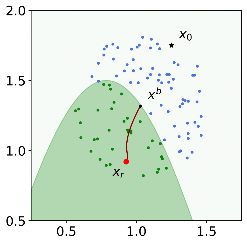
Figure 1: An example of the robust Bayesian recourse on a toy 2-dimensional instance. The star denotes the input , and the black circle denotes the boundary point . Green and blue circles are locally sampled data with favorable and unfavorable predicted values, respectively. The red circle denotes the robust Bayesian recourse, and the curved line denotes the continuum of intermediate solutions of the gradient descent algorithm. The robust Bayesian recourse moves to the interior of the favorable region (green), and thus is more likely to be valid subject to model shifts.
4. Wasserstein-Gaussian Mixture Ambiguity Sets
A central problem in solving the robust Bayesian recourse is how to construct the ambiguity set . Our construction relies on representing a Gaussian mixture distribution as a discrete distribution on the mean vector and covariance matrix space.
Notice that the smoothed measure is a Gaussian mixture and any Gaussian distribution is fully characterized by its mean vector and its covariance matrix. Thus, is associated with the discrete distribution  on the space of mean vector and covariance matrix
  .
.
Then, for any  , we formally define the ambiguity set as
![\[\mathbb{B}_{\varepsilon_y}(\hat{\mathbb{P}}_y^\sigma) \triangleq \left\{ \mathbb{Q}_y: \begin{array}{l} \nu_y \in \mathcal{P}(\mathbb{R}^p \times \mathbb{S}_{\geq\sigma}^p),~\mathbb{W}_c(\nu_y, \widehat{\nu}_y) \leq \varepsilon_y \\ \mathbb{Q}_y \text{ is a Gaussian mixture associated with } \nu_y \end{array}\right\}.\]](https://research.vinai.io/wp-content/ql-cache/quicklatex.com-fe2c7098525217534b8ebdf840f31f80_l3.svg "Rendered by QuickLaTeX.com")
Here,  is the set of covariance matrices whose eigenvalues are lower bounded by
  , with
  is the isotropic variance of the smoothing convolution.
  denotes the set of all possible distributions supported on
  .
.
Intuitively, contains all Gaussian mixtures  associated with some
  having a distance less than or equal to
  from the nominal measure
  . The distance between and is measured by an optimal transport
  .
.
Particularly, we use as the type- Wasserstein distance, which differentiates us from the literature whose focuses are type-1 and type-2 distances [4, 5]. This type- construction is critical for the computational tractability of our problem.
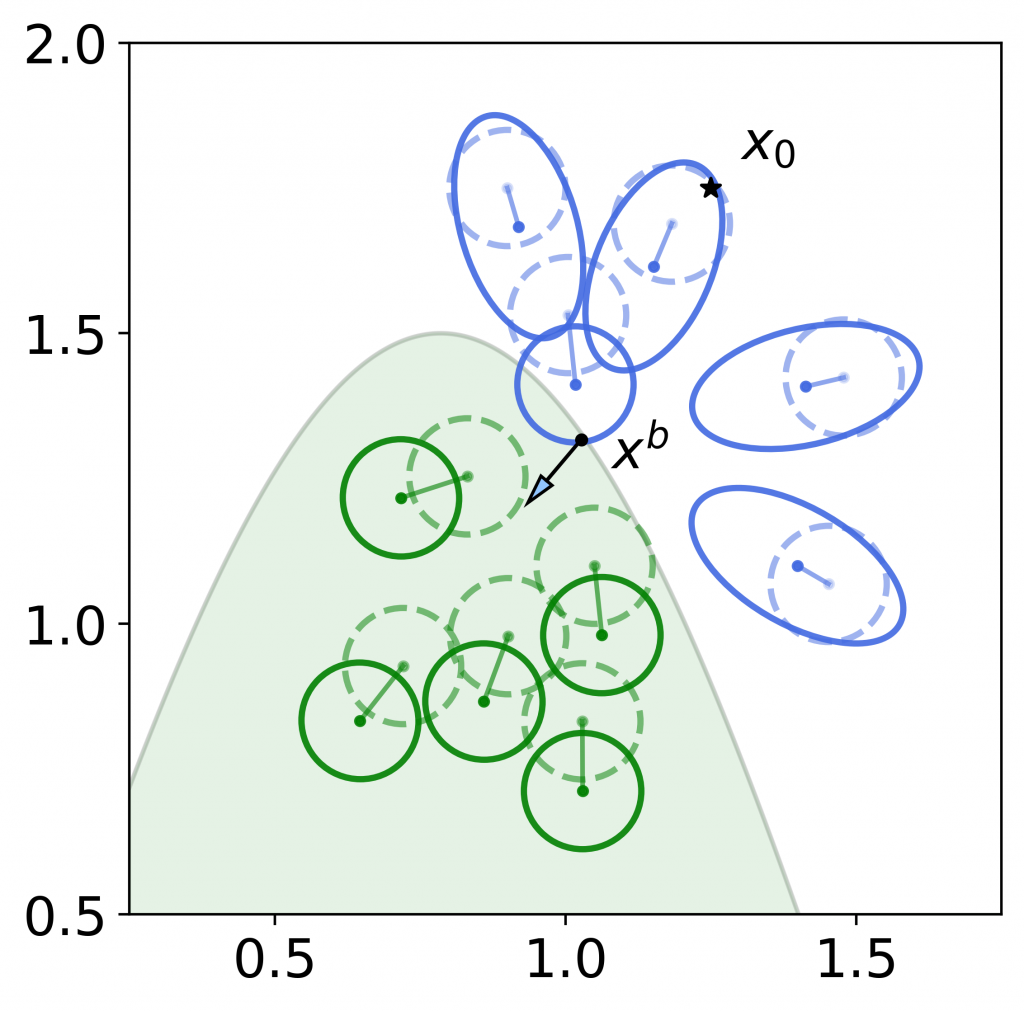
Figure 2: Another visualization of the worst-case distributions on a toy dataset. The dashed, opaque dots and circles represent the isotropic Gaussian around each data sample. The solid dots and circles represent the worst-case distributions corresponding to the boundary point . For blue (unfavorably predicted) samples, the worst-case distribution is formed by perturbing the distribution towards — which leads to maximizing the posterior probability of unfavorable prediction. For green (favorably predicted) samples, the worst-case distribution is formed by perturbing the distribution away from — which leads to minimizing the posterior probability of favorable prediction. These worst-case distributions will maximize the posterior probability odds ratio.
5. Reformulation of the likelihood evaluation problems
In the paper, by leveraging the essential supremum in the definition of the type- Wasserstein distance, we prove that the evaluation of the optimistic and pessimistic likelihoods can be decomposed into solving smaller subproblems, and that each is an optimization problem over the mean vector – covariance matrix space .
We further show that each of these subproblems can be reduced to a 2-dimensional subproblem independent of the original dimension  .
.
For the sake of brevity, we only state here the final reformulations of our likelihood evaluation problems. Interested readers are welcome to read our papers for the full derivation.
Optimistic likelihood
For each  , let
, let  be the optimal value of the following two-dimensional optimization problem
![\[\min_{\substack{a \in \mathbb{R}_+,~d_p \in [\sigma, +\infty) \\ a^2 + (d_p - \sigma)^2 \leq \epsilon_0^2 }} ~\left\{\log d_p + \frac{(\|x - \widehat{x}_i\|_2 - a)^2}{2d_p^2} + (p-1) \log \sigma\right\}.\]](https://research.vinai.io/wp-content/ql-cache/quicklatex.com-5980e6578f036ac81f13837a7810a0fd_l3.svg "Rendered by QuickLaTeX.com")
Then, we have
![\[\max~\{ L(x, \mathbb{Q}_0) : \mathbb{Q}_0 \in \mathbb{B}{\varepsilon_0}(\hat{\mathbb{P}}_0^\sigma)\} = \frac{\sum_{i \in \mathcal{I}_0} \exp(-\alpha_i)}{N_0 (2\pi)^{p/2}}.\]](https://research.vinai.io/wp-content/ql-cache/quicklatex.com-18bc50ee4dcacd3ec401a81cd98d0141_l3.svg "Rendered by QuickLaTeX.com")
Pessimistic likelihood
For each  , let be the optimal value of the following two-dimensional optimization problem
![\[\min_{\substack{a \in \mathbb{R}_+,~d_1 \in [\sigma, +\infty)\\ a^2 + p(d_1 - \sigma)^2 \leq \epsilon_1^2}} ~ \left\{-\log d_1 - \frac{(\|x - \widehat{x}_i\|_2 + a)^2}{2d_1^2} - (p-1) \log \left(\sigma + \sqrt{\frac{\epsilon_1^2 - a^2 - (d_1 - \sigma)^2}{p - 1}}\right) \right\}.\]](https://research.vinai.io/wp-content/ql-cache/quicklatex.com-f937ba09175995268b3413ed337b3e97_l3.svg "Rendered by QuickLaTeX.com")
Then we have
![\[\max~\{ L(x, \mathbb{Q}_1) : \mathbb{Q}_1 \in \mathbb{B}_{\varepsilon_1}(\hat{\mathbb{P}}_1^\sigma)\} = \frac{\sum_{i \in \mathcal{I}_1} \exp(-\alpha_i)}{N_1 (2\pi)^{p/2}}.\]](https://research.vinai.io/wp-content/ql-cache/quicklatex.com-190d49545fd31f93a0649d715b6fcba4_l3.svg "Rendered by QuickLaTeX.com")
with the above theorems, we can design an iterative scheme to solve the robust Bayesian recourse problem. For any value , we can use projected gradient descent to solve a series of two-dimensional subproblems to evaluate the objective value .
6. Experiments
We evaluate the robustness of our method to model shifts of different recourses, together with the trade-off against the cost of adopting the recourse’s recommendation. We compare our proposed robust Bayesian recourse (RBR) method against the counterfactual explanations of Wachter, and ROAR robust recourses generated using either LIME and LIMES surrogate models.
Experimental setup
Datasets
We examine the recourse generators on both a synthetic dataset and the real-world datasets: German Credit [6, 7] Small Bussiness Administration (SBA) [8], and Give Me Some Credit (GMC) [9]. Each dataset contains two sets of data:  and
and  . The former is the current data which is used to train a current classifier to generate recourses. The latter represents the possible data arriving in the future.
For each dataset, we use 80% of the instances in the current data to train the underlying predictive model and fix this classifier to construct recourses for the remaining 20% of the instances. The future data will be used to train future classifiers, which are for evaluation only.
Classifier
We use a three-layer MLP with 20, 50 and 20 nodes, respectively with a ReLU activation in each consecutive layer. The sigmoid function is used in the last layer to produce predictive probabilities. The performance of the MLP classifier is reported in Table 1 below.
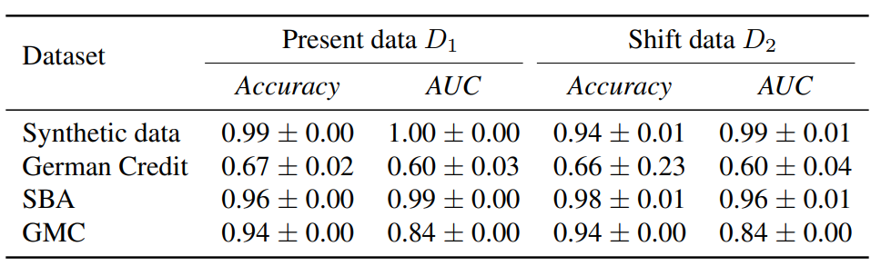
Table 1. Accuracy and AUC results of the MLP classifier on the synthetic and real-world datasets
Metrics
To measure the ease of adopting a recourse, we use the  -distance as the cost function on the covariate space , this choice is similar to [3] and [10]. We define the current validity as the validity of the recourses with respect to the current classifier
  . To evaluate the robustness of recourses to the changes in model’s parameters, we sample 20% of the instances in the data set as the arrival data. We then re-train the classifier with the old data (80% of ) coupled with this arrival data to simulate the future classifiers
  . We repeat this procedure 100 times to obtain 100 future classifiers and report the future validity of a recourse as the fraction of the future classifiers with respect to which the recourse is valid.
Readers are welcome to read our paper for more details on the experiments.
Cost-validity trade-off
We obtain the Pareto front for the trade-off between the cost of adopting recourses produced by RBR and their validity by varying the ambiguity sizes  and
and  , along the maximum recourse cost
  . Particularly, we consider
  and
and 
The frontiers for ROAR-based methods are obtained by varying  , where
  is the tuning parameter of ROAR.
As shown in the figure below, increasing and  generally increase the future validity of recourses yielded by RBR at the sacrifice of the cost, while sustaining the current validity. Yet, the frontiers obtained by RBR either dominate or are comparable to other frontiers of Wachter, LIME-ROAR, and LIMELS-ROAR.
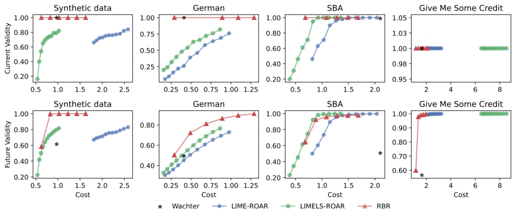
Figure 3. Pareto frontiers of the cost-validity trade-off with the MLP classifier, on synthetic, German Credit, Small Business Administration, and Give Me Some Credit datasets.
7. References
[1] Alexandre B. Tsybakov. Introduction to Nonparametric Estimation. Springer, 2008.
[2] Suresh Venkatasubramanian and Mark Alfano. The philosophical basis of algorithmic recourse. In Proceedings of the 2020 Conference on Fairness, Accountability, and Transparency, page 284–293, 2020.
[3] Sohini Upadhyay, Shalmali Joshi, and Himabindu Lakkaraju. Towards robust and reliable algorithmic recourse. In Advances in Neural Information Processing Systems, 2021.
[4] Viet Anh Nguyen, Soroosh Shafieezadeh-Abadeh, ManChung Yue, Daniel Kuhn, and Wolfram Wiesemann. Calculating optimistic likelihoods using (geodesically) convex optimization. In Advances in Neural Information Processing Systems 32, pages 13942–13953, 2019.
[5] Viet Anh Nguyen, Nian Si, and Jose Blanchet. Robust Bayesian classification using an optimistic score ratio. In Proceedings of the 37th International Conference on Machine Learning, 2020.
[6] Dheeru Dua and Casey Graff. UCI machine learning repository, 2017. URL http://archive.ics.uci.edu/ml
[7] U Groemping. South German credit data: Correcting a widely used data set. Reports in Mathematics, Physics and Chemistry, Department II, Beuth University of Applied Sciences Berlin, 2019.
[8] Min Li, Amy Mickel, and Stanley Taylor. “Should this loan be approved or denied?”: A large dataset with class assignment guidelines. Journal of Statistics Education, 26(1):55–66, 2018.
[9] Kaggle Competition. Give me some credit. improve on the state of the art in credit scoring by predicting the probability that somebody will experience financial distress in the next two years., 2011. URL https://www.kaggle.com/competitions/GiveMeSomeCredit/data
[10] Berk Ustun, Alexander Spangher, and Yang Liu. Actionable recourse in linear classification. In Proceedings of the Conference on Fairness, Accountability, and Transparency, pages 10–19, 2019.