Introduction
The recent advance in computation of optimal transport has led to a surge of interest in applying this tool in machine learning and data science, including deep generative models [1], domain adaptation [2], etc. In these applications, optimal transport provides a metric, named Wasserstein distance, to quantify the discrepancy of the locations and mass between two probability measures defined in the same space. When input probability measures lie in different spaces, Gromov-Wasserstein distance is adopted to measure the discrepancy between their inner structures. However, this metric is computationally expensive as it requires us to solve a quadratic programming problem. Therefore, we consider its entropic version, called entropic Gromov-Wasserstein, where we add a relative entropy term to the objective function in order to reduce the computational cost.
Related work
Salmona et.la [3] have studied the Gromov-Wasserstein distance between Gaussian distributions using L2-norm cost functions. In that paper, they can only derive upper and lower bounds for the Gromov-Wasserstein distance without explicitly showing its closed-form expression. This is due to the dependence on co-moments of order 2 and 4 of feasible transport plans (see Theorem 2.1, [3]). Moreover, they are not even able to demonstrate that an optimal transport plan is a Gaussian distribution. Thus, we investigate in this work an entropic inner-product Gromov-Wasserstein problem and its unbalanced variant between (unbalanced) Gaussian distributions, which can be regarded as the first step to gain a better understanding and new insights on the L2-norm Gromov-Wasserstein distance. Additionally, we also study its corresponding barycenter problem among multiple Gaussian distributions.
Entropic Gromov-Wasserstein between balanced Gaussians
In this section, we present a closed-form expression of the entropic inner-product Gromov-Wasserstein (entropic IGW) between two Gaussian measures. It can be seen from Theorem 3.1 that this expression depends only on the eigenvalues of covariance matrices of two input measures. Interestingly, as the regularization parameter goes to zero, the closed form of the entropic IGW converges to the squared Euclidean distance between these two covariance matrices, reflecting the difference in the inner structures of two input measures. Our key ingredient lies in Lemma 3.4 where we utilize the von Neumann’s trace inequality, which says that the sum of singular values of the product of two matrices is maximized when their singular value decompositions share the same orthogonal bases and and their corresponding singular values match that of each other by their magnitudes. Furthermore, we show that a corresponding optimal transport plan is also a Gaussian distribution by utilizing a nice geometric property of the entropic regularization term (see Lemma 3.3).
Next, we will use the derived closed-form to examine the behavior of algorithms studied in [4] for solving the entropic Gromov-Wasserstein problem. Here, we set the dimensions of spaces of two input measures to be 2 and 3. Then, we sample N (between 10 and 2000) data points from two corresponding zero-mean Gaussian distributions with diagonal covariance matrices whose diagonal entries are uniformly sampled from the interval [0, 2]. The regularization parameter is chosen among three values 0.5, 1 and 5. We plot means and one standard deviation areas over 20 independent runs for each value of N as follows.
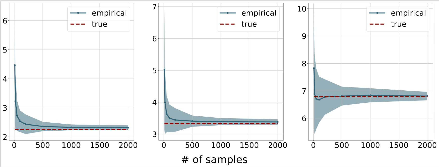
Figure 1. Empirical convergence for the algorithm in [4]. From left to right: the regularization parameters are 0.5, 1 and 5. The red dash lines correspond to the theoretical optimal values, while the blue lines and shaded regions are the means and standard deviations of the objective values computed according to [4], respectively.
As expected, with more samples, we can approximate the entropic IGW more accurately.
Entropic Unbalanced Gromov-Wasserstein between unbalanced Gaussians
When the two input measures are unbalanced Gaussians, i.e. their total masses could be different, the aforementioned entropic IGW formulation is no longer valid. Therefore, we introduce a new variant, named entropic unbalanced IGW (entropic UIGW), by relaxing marginal constraints via Kullback-Leibler (KL) divergence. Nevertheless, the involvement of two new KL divergence terms in the objective function causes many challenges in deriving a closed form for the entropic UIGW. To overcome that difficulty, we introduce a lower bound for the KL divergence between two Gaussian distributions in Lemma 4.1. Based on that result, we show that the objective function can be broken down into several sub-problems that can be solved explicitly through some quadratic and cubic equations. This leads to an almost closed-form expression of the Gaussian optimal transport plan of the entropic UIGW between unbalanced Gaussian measures in Theorem 4.2.
Similar to the previous section, we use the same setting and the closed form for the unbalanced formulation to demonstrate the convergence of the algorithm 1 in [5], which solves a bi-convex relaxation of the entropic UIGW problem. In addition, the KL regularization parameter is set to 1. It can be seen from the following figure that the approximation quality increases when there are more samples.
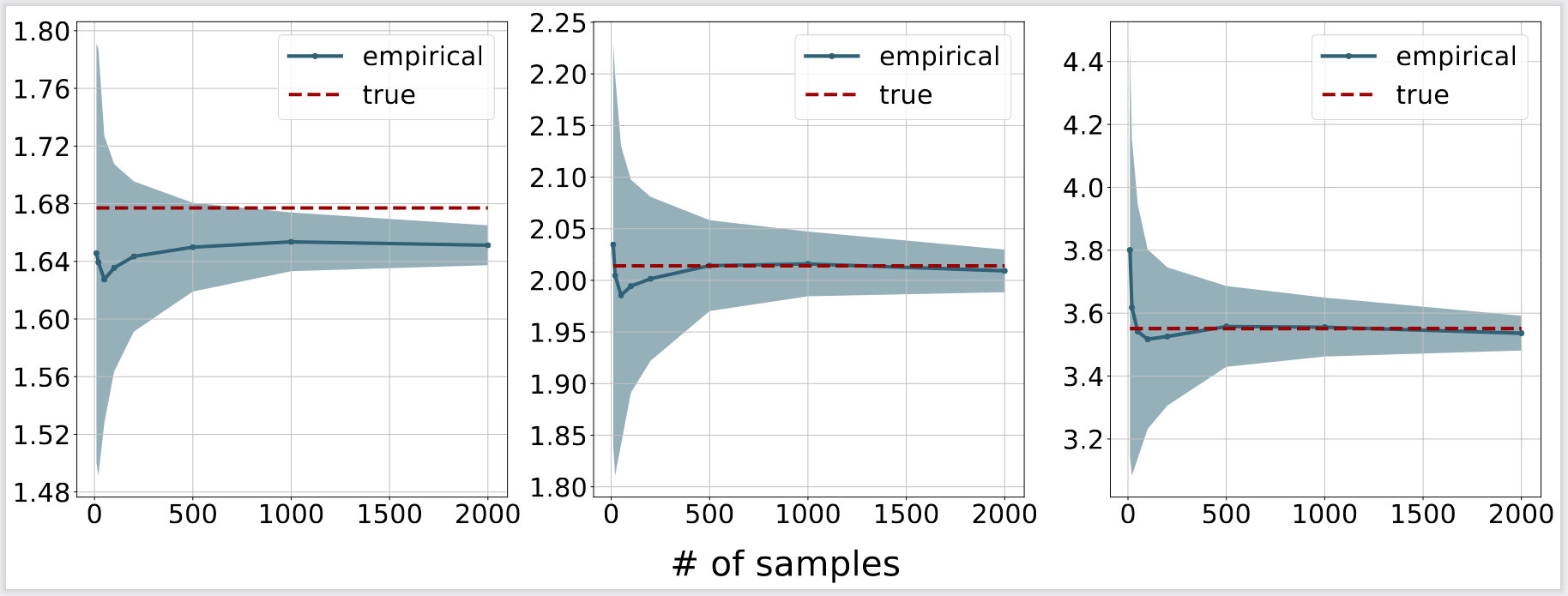
Figure 2. Empirical convergence for the algorithm in [5]. From left to right: the regularization parameters are 0.5, 1 and 5. The red dash lines correspond to the theoretical optimal values, while the blue lines and shaded regions are the means and standard deviations of the objective values computed according to [5], respectively.
(Entropic) Gromov-Wasserstein Barycenter of Gaussians
Subsequently, we consider the problem of computing the (entropic) Gromov-Wasserstein barycenter of T Gaussian measures defined in spaces of various dimensions. To tackle this problem, it is necessary to fix the desired dimension of a barycenter, and choose beforehand positive weighting coefficients associated with given measures. Next, we prove that the barycenter of Gaussian measures is also a Gaussian measure with a diagonal covariance matrix, and then successfully extend this interesting result to the entropic version when the regularization parameter is sufficiently small, which is a widely used setting in practice.
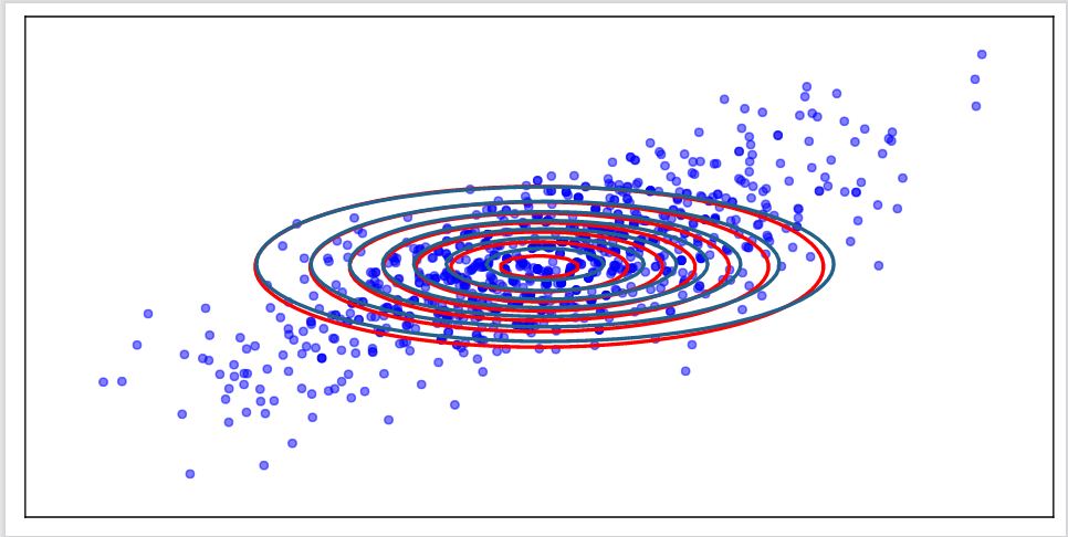
Figure 3. Visualizing the barycenter. The blue points correspond to one possible set of support for the computed barycenter by [4]. The blue contours are the rotated version of the Gaussian fitted to this support set (for comparison). The red contours represent the theoretical barycenter whose form is presented in Theorem 5.4.
References
[1] Arjovsky, M., Chintala, S., and Bottou, L. Wasserstein generative adversarial networks. In International Conference on Machine Learning, pp. 214–223, 2017.
[2] Courty, N., Flamary, R., Tuia, D., and Rakotomamonjy, A. Optimal transport for domain adaptation. IEEE transactions on pattern analysis and machine intelligence, 39(9): 1853–1865, 2016.
[3] Salmona, A., Delon, J., and Desolneux, A. GromovWasserstein distances between Gaussian distributions. Arxiv Preprint Arxiv: 2104.07970, 2021.
[4] Peyré, G., Cuturi, M., and Solomon, J. Gromov-Wasserstein averaging of kernel and distance matrices. In International Conference on Machine Learning, pp. 2664–2672, 2016.
[5] Séjourné, T., Vialard, F.-X., and Peyré, G. The unbalanced gromov-wasserstein distance: Conic formulation and relaxation. In Advances in Neural Information Processing Systems, 2021.