1. Introduction
The central question of transfer learning from one domain to another domain is how could we ensure good performance of the model on the test domain, given the model having good performance on the training domain. Here, a domain is defined generally as a joint distribution on data-label space. Depending on the availability of the target domain during training, we encounter either multiple source domain adaptation (MSDA) or domain generalization (DG) problem.
Domain adaptation (DA) is a specific case of MSDA when we need to transfer from a single source domain to another target domain available during training. For the DA setting, domain-invariant (DI) representations are thoroughly studied [1]: what is it, how to learn this kind of representations [3], and the trade-off of enforcing learning DI representations [6].
On the other hand, due to the presence of multiple source domains and possibly unavailability of target domain, establishing theoretical foundation and characterizing DI representations for the MSDA and especially DG settings are significantly more challenging. Moreover, previous works [1, 5, 4, 7, 6] do not investigate the DI representations under a representation learning viewpoint. The common approach is connecting loss on target domain to divergence of data distribution, labelling function mismatch, and loss on source domain, without any mention of representation. On the other hand, we argue that the representation must be explicitly discussed in order to conclude anything about the DI representation.
2. Main Theory
2.1. Notations
Let  be a data space,
  be a data distribution on this space, and
  be the corresponding density function We consider the multi-class classification problem with the label set
 ![\mathcal{Y}=\left[C\right]](https://research.vinai.io/wp-content/ql-cache/quicklatex.com-90d2913336adbe3c74ad115adaa7dae8_l3.svg "Rendered by QuickLaTeX.com") , where
, where  is the number of classes and
 ![\left[C\right]:=\{1,\ldots,C\}](https://research.vinai.io/wp-content/ql-cache/quicklatex.com-eb2a40c810cf65d9905517fae094dccd_l3.svg "Rendered by QuickLaTeX.com") . Denote
. Denote  as the
  simplex label space, let
  be a probabilistic labeling function returning a -tuple
 ![f\left(x\right)=\left[f\left(x,i\right)\right]_{i=1}^{C}](https://research.vinai.io/wp-content/ql-cache/quicklatex.com-63e4747a08a172c82e3491be6f019e42_l3.svg "Rendered by QuickLaTeX.com") , whose element
, whose element  is the probability to assign a data sample
  to the class
  (i.e.,
  ). Moreover, a domain is denoted compactly as pair of data distribution and labeling function
  . We note that given a data sample , its categorical label
  is sampled as
  which a categorical distribution over
  .
.
Let  be a loss function. The general loss of a classifier
  on a domain
  is
is
![\[ \mathcal{L}\left(\hat{f},f,\mathbb{P}\right)=\mathcal{L}\left(\hat{f},\mathbb{D}\right):=\mathbb{E}_{x\sim\mathbb{P}}\left[\ell\left(\hat{f}(x),f(x)\right)\right]. \]](https://research.vinai.io/wp-content/ql-cache/quicklatex.com-ecd241397f220a56b40a83d9b0bc4f01_l3.svg "Rendered by QuickLaTeX.com")
We inspect the multiple source setting in which we are given multiple source domains  over the common data space , each of which consists of data distribution and its own labeling function
  . When combining the source domains, we obtain a mixture of multiple source distributions denoted as
  , where the mixing coefficients
 ![\pi=\left[\pi_{i}\right]_{i=1}^{K}](https://research.vinai.io/wp-content/ql-cache/quicklatex.com-b937e3bfe63f78f2a3f5621068d1b8e5_l3.svg "Rendered by QuickLaTeX.com") can be conveniently set to
can be conveniently set to  with
with  being the training size of the
  th source domain. Similarly, the target domain is
  .
.
To this end, previous works generally upper bound the target loss using sum of source loss, a divergence term between source and target data distributions, and a constant involving labeling functions of source and target domains.
![\[ \mathcal{L}\left(\hat{f},\mathbb{D}^{T}\right)\leq\sum_{i=1}^{K}\pi_{i}\mathcal{L}\left(\hat{f},\mathbb{D}^{S,i}\right)+D\left(\sum_{i=1}^{K}\pi_{i}\mathbb{P}^{S,i},\mathbb{P}^{T}\right)+\lambda \]](https://research.vinai.io/wp-content/ql-cache/quicklatex.com-39c8ea2e77751024f7881047cbf89619_l3.svg "Rendered by QuickLaTeX.com")
From this formulation, learning DI representation is said to be encouraged via minimizing the divergence  , but on the representation space, e.g.,
 denoting representation distribution). However, we argue that this formulation is not explicit and concrete for discussing DI representation learning.
In our setting, input is mapped into a latent space  by a feature map
  , and then a classifier
  is trained based on the representations
  . Let be the original labeling function. To facilitate the theory developed for latent space, we introduce representation distribution being the pushed-forward distribution
  , and the labeling function
  induced by
  as
as  . Going back to our multiple source setting, the source mixture becomes
  , where each source domain is
  , and the target domain is
  .
.
Finally, in our theory development, we use Hellinger divergence between two distributions defined as  , whose squared
  is a proper metric.
2.2. Two types of representation
(1) ![\begin{equation*}</em> <em>\begin{aligned}\mathcal{L}\left(\hat{f},\mathbb{D}^{T}\right)\leq\sum_{i=1}^{K}\pi_{i}\mathcal{L}\left(\hat{f},\mathbb{D}^{S,i}\right)+L\max_{i\in[K]}\mathbb{E}_{\mathbb{P}^{S,i}}\left[\|\Delta p^{i}(y|x)\|_{1}\right]+L\sqrt{2}\,d_{1/2}\left(\mathbb{P}_{g}^{T},\mathbb{P}_{g}^{\pi}\right)\end{aligned}</em> <em></em> <em>\end{equation*}](https://research.vinai.io/wp-content/ql-cache/quicklatex.com-524e8fdef7198d817abf44787e8c371b_l3.svg "Rendered by QuickLaTeX.com")
where ![\Delta p^{i}(y|x):=\left[\left|f^{T}(x,y)-f^{S,i}(x,y)\right|\right]_{y=1}^{C}](https://research.vinai.io/wp-content/ql-cache/quicklatex.com-5be3280f9b981163858e2c19527cdcb7_l3.svg "Rendered by QuickLaTeX.com") is the absolute of single point label shift on input space between source domain
is the absolute of single point label shift on input space between source domain  , the target domain
  , and
, and ![[K]:=\left\{ 1,2,...,K\right\}](https://research.vinai.io/wp-content/ql-cache/quicklatex.com-91d113e483e74082d59c24162a820838_l3.svg "Rendered by QuickLaTeX.com") .
.
The bound in Equation 1 implies that the target loss in the input or latent space depends on three terms: (i) representation discrepancy:  , (ii) the label shift:
 ![\max_{i\in[K]}\mathbb{E}_{\mathbb{P}^{S,i}}\left[\|\Delta p^{i}(y|x)\|_{1}\right]](https://research.vinai.io/wp-content/ql-cache/quicklatex.com-77f765042bb32c351b1ea1247ab73074_l3.svg "Rendered by QuickLaTeX.com") , and (iii) the general source loss:
, and (iii) the general source loss:  . To minimize the target loss in the left side, we need to minimize the three aforementioned terms. First, the \emph{label shift} term is a natural characteristics of domains, hence almost impossible to tackle. Secondly, the representation discrepancy term can be explicitly tackled for the MSDA setting, while almost impossible for the DG setting. Finally, the general source loss term is convenient to tackle, where its minimization results in a feature extractor and a classifier
  .
.
Contrary to previous works in DA and MSDA [1, 5, 7, 2] that consider both losses and data discrepancy on data space, our bound connects losses on data space to discrepancy on representation space. Therefore, our theory provides a natural way to analyse representation learning, especially feature alignment in deep learning practice. Note that although DANN [3] explains their feature alignment method using theory developed by Ben-david et al. [1], it is not rigorous. In particular, while application of the theory to representation space yield a representation discrepancy term, the loss terms are also on that feature space, and hence minimizing these losses is not the learning goal. Finally, our setting is much more general, which extends to multilabel, stochastic labeling setting, and any bounded loss function.
As the final piece, the representation discrepancy can be broken down as  . To this end, we could define two types of DI representation.
ii) (Compressed Domain-Invariant Representation) A feature map  is a DG compressed DI representations for source domains if
  is the solution of the optimization problem (OP):
  which satisfies
(i.e., the pushed forward distributions of all source domains are identical). The latent representations  is then called compressed DI representations for the DG setting.
2.3. Trade-off bound
Similar to the theoretical finding in Zhao et al. 2019 [6] developed for DA, we theoretically find that compression does come with a cost for MSDA and DG. We investigate the representation trade-off, typically how compressed DI representation affects classification loss. Specifically, we consider a data processing chain  , where is the common data space, is the latent space induced by a feature extractor , and is a hypothesis on top of the latent space. We define
  and
and  as two distribution over
  in which to draw
  , we sample
  ,
,  , and
, and  , while similar to draw
  . Our theoretical bounds developed regarding the trade-off of learning DI representations are relevant to
  .
.
![d_{1/2}\left(\mathbb{P}_{\mathcal{Y}}^{\pi},\mathbb{P}_{\mathcal{Y}}^{T}\right)\leq\left[\sum_{k=1}^{K}\pi_{k}\mathcal{L}\left(\hat{h}\circ g,f^{S,k},\mathbb{P}^{S,k}\right)\right]^{1/2}+d_{1/2}\left(\mathbb{P}_{g}^{T},\mathbb{P}_{g}^{\pi}\right)+\mathcal{L}\left(\hat{h}\circ g,f^{T},\mathbb{P}^{T}\right)^{1/2}](https://research.vinai.io/wp-content/ql-cache/quicklatex.com-cdde3c679cb3aad295e876362dd98cc6_l3.svg "Rendered by QuickLaTeX.com")
![d_{1/2}\left(\mathbb{P}_{\mathcal{Y}}^{\pi},\mathbb{P}_{\mathcal{Y}}^{T}\right)\leq\left[\sum_{i=1}^{K}\pi_{i}\mathcal{L}\left(\hat{h}\circ g,f^{S,i},\mathbb{P}^{S,i}\right)\right]^{1/2}+\sum_{i=1}^{K}\sum_{j=1}^{K}\frac{\sqrt{\pi_{j}}}{K}d_{1/2}\left(\mathbb{P}_{g}^{S,i},\mathbb{P}_{g}^{S,j}\right)+\sum_{i=1}^{K}\sum_{j=1}^{K}\frac{\sqrt{\pi_{j}}}{K}d_{1/2}\left(\mathbb{P}_{g}^{T},\mathbb{P}_{g}^{S,i}\right)+\mathcal{L}\left(\hat{h}\circ g,f^{T},\mathbb{P}^{T}\right)^{1/2}.](https://research.vinai.io/wp-content/ql-cache/quicklatex.com-57d091529b7199dbbfed838353f342fa_l3.svg "Rendered by QuickLaTeX.com")
Here we note that the general loss  is defined based on the Hellinger loss
  which is define as
  (more discussion can be found in Appendix C).
Remark. Compared to the trade-off bound in the work of Zhao et al. 2019, our context is more general, concerning MSDA and DG problems with multiple source domains and multi-class probabilistic labeling functions, rather than single source DA with binary-class and deterministic setting.
Moreover, the Hellinger distance is more universal, in the sense that it does not depend on the choice of classifier family  and loss function as in the case of -divergence in Theorem [1].
We base on the first inequality of Theorem [3] to analyze the trade-off of learning general DI representations. The first term on the left hand side is the source mixture’s loss, which is controllable and tends to be small when enforcing learning general DI representations. With that in mind, if \textit{two label marginal distributions } and are distant (i.e., is high), the sum  tends to be high. This leads to 2 possibilities. The first scenario is when the representation discrepancy has small value, e.g., it is minimized in MSDA setting, or it happens to be small by pure chance in DG setting. In this case, the lower bound of target loss
  is high, possibly hurting model’s generalization ability. On the other hand, if the discrepancy is large for some reasons, the lower bound of target loss will be small, but its upper-bound is higher, as indicated in Theorem [1].
Based on the second inequality of Theorem [3], we observe that if two label marginal distributions and are distant while enforcing learning
compressed DI representations (i.e., both source loss and source-source feature discrepancy ![\left[\sum_{i=1}^{K}\pi_{i}\mathcal{L}\left(\hat{h}\circ g,f^{S,i},\mathbb{P}^{S,i}\right)\right]^{1/2}+\sum_{i=1}^{K}\sum_{j=1}^{K}\frac{\sqrt{\pi_{j}}}{K}d_{1/2}\left(\mathbb{P}_{g}^{S,i},\mathbb{P}_{g}^{S,j}\right)](https://research.vinai.io/wp-content/ql-cache/quicklatex.com-944a899d4bc2944acf550ae4d083c794_l3.svg "Rendered by QuickLaTeX.com")
are low), the sum  is high. For the MSDA setting, the discrepancy
  is trained to get smaller, meaning that the lower bound of target loss is high, hurting the target performance. Similarly, for the DG setting, if the trained feature extractor occasionally reduces for some unseen target domain, it certainly increases the target loss
  . In contrast, if for some target domains, the discrepancy is high by some reasons, by linking to our upper bound, the target general loss has a high upper-bound, hence is possibly high.
This trade-off between representation discrepancy and target loss suggests a sweet spot for just-right feature alignment. In that case, the target loss is most likely to be small.
Experiments
We wish to study the characteristics and trade-off between two kinds of DI representations when predicting on various target domains. Specifically, we apply adversarial learning similar to {[}Ganin et al. 2016{]}, in which a min-max game is played between domain discriminator  trying to distinguish the source domain given representation, while the feature extractor (generator) tries to fool the domain discriminator. Simultaneously, a classifier is used to classify label based on the
representation. Let  and
and  be the label classification and domain discrimination losses, the training objective becomes:
![\[ \min_{g}\left(\min_{\hat{h}}\mathcal{L}_{gen}+\lambda\max_{\hat{h}^{d}}\mathcal{L}_{disc}\right), \]](https://research.vinai.io/wp-content/ql-cache/quicklatex.com-437477da5782b8eb9f5e9ba8fa975e03_l3.svg "Rendered by QuickLaTeX.com")
where the source compression strength  controls the compression extent of learned representation. More specifically, general DI representation is obtained with
  , while larger
  leads to more compressed DI representation. We did experiments on a CMNIST dataset and a real-world dataset PACS, whose details are in our official paper. Finally, our implementation is based on DomainBed repository.
Figure 1a shows the source validation and target accuracies when increasing (i.e., encouraging the source compression). It can be observed that both source validation accuracy and target accuracy have the same pattern: increasing when setting appropriate for just-right compressed DI representations and compromising when setting overly high values for overly-compressed DI representation. Figure 1b shows in detail the variation of the source validation accuracy for each specific . In practice, we should encourage learning two kinds of DI representations simultaneously by finding an appropriate trade-off to balance them for working out just-right compressed DI representations.
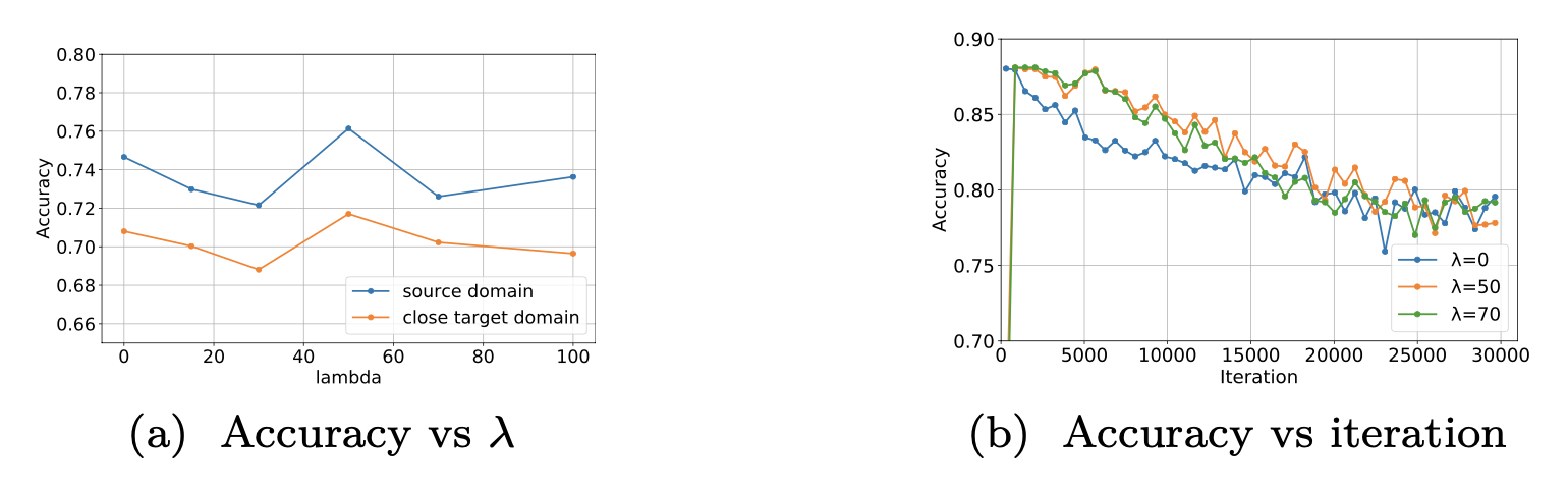
Figure 1: (CMNIST) (1a) Source validation accuracy and target accuracy for target domain w.r.t. compression strength. (1b) Validation accuracy over training step for different values of λ.
[1] Ben-David, S., Blitzer, J., Crammer, K., Kulesza, A., Pereira, F., and Vaughan, J. W. A theory of learning from different domains. Mach. Learn. 79, 1–2 (May 2010), 151–175. 1, 2.2
[2] Cortes, C., Mohri, M., and Medina, A. M. Adaptation based on generalized discrepancy. Journal of Machine Learning Research 20, 1 (2019), 1–30. 2.2
[3] Ganin, Y., Ustinova, E., Ajakan, H., Germain, P., Larochelle, H., Laviolette, F., March, M., and Lempitsky, V. Domain-adversarial training of neural networks. Journal of Machine Learning Research 17, 59 (2016), 1–35. 1, 2.2
[4] Hoffman, J., Mohri, M., and Zhang, N. Algorithms and theory for multiple-source adaptation. In Advances in Neural Information Processing Systems (2018), S. Bengio, H. Wallach, H. Larochelle, K. Grauman, N. Cesa- Bianchi, and R. Garnett, Eds., vol. 31, Curran Associates, Inc. 1
[5] Mansour, Y., Mohri, M., and Rostamizadeh, A. Domain adaptation with multiple sources. In Advances in Neural Information Processing Systems (2009), D. Koller, D. Schuurmans, Y. Bengio, and L. Bottou, Eds., vol. 21, Curran Associates, Inc. 1, 2.2
[6] Zhao, H., Combes, R. T. D., Zhang, K., and Gordon, G. On learning invariant representations for domain adaptation. In Proceedings of the 36th International Conference on Machine Learning (09–15 Jun 2019), K. Chaud- huri and R. Salakhutdinov, Eds., vol. 97 of Proceedings of Machine Learning Research, PMLR, pp. 7523–7532. 1, 2.3, 2.3
[7] Zhao, H., Zhang, S., Wu, G., Moura, J. M. F., Costeira, J. P., and Gordon, G. J. Adversarial multiple source domain adaptation. In Advances in Neural Information Processing Systems (2018), S. Bengio, H. Wallach, H. Larochelle, K. Grauman, N. Cesa-Bianchi, and R. Garnett, Eds., vol. 31, Curran Associates, Inc. 1, 2.2
 . For any hypothesis
  with
with  . Moreover, the latent representations